
Assumptions in Linear Regression
- 7rishi20ss
- Feb 26, 2023
- 8 min read

This post is going to about what are the assumptions inline regression and how do we find if those assumptions hold and if not how can we correct them.
So to get started we are doing this on dataset called Boston Housing Dataset, which is good dataset to start with if you are learning linear regression.
Description of Dataset
The Boston Housing Dataset is derived from data gathered by the U.S. Census Service about housing in the Boston, Massachusetts, area. The columns of the dataset are described as follows:
CRIM - per capita crime rate by town
ZN - proportion of residential land zoned for lots over 25,000 sq.ft.
INDUS - proportion of non-retail business acres per town.
CHAS - Charles River dummy variable (1 if tract bounds river; 0 otherwise)
NOX - nitric oxides concentration (parts per 10 million)
RM - average number of rooms per dwelling
AGE - proportion of owner-occupied units built prior to 1940
DIS - weighted distances to five Boston employment centres
RAD - index of accessibility to radial highways
TAX - full-value property-tax rate per $10,000
PTRATIO - pupil-teacher ratio by town
B - 1000(Bk - 0.63)^2 where Bk is the proportion of blacks by town
LSTAT - % lower status of the population
MEDV - Median value of owner-occupied homes in $1000's
you can find the dataset on Kaggle.
Now let's get started.
Assumptions in Linear Regression
Linear regression makes several assumptions about the data, and violating these assumptions can lead to biased or inaccurate estimates of the regression coefficients. Here are the main assumptions of linear regression
Linearity : The relationship between the independent variable(s) and the dependent variable is linear. This means that the change in the dependent variable is proportional to the change in the independent variable(s).
Independence: The observations in the dataset are independent of each other. In other words, the value of the dependent variable for one observation should not be influenced by the value of the dependent variable for another observation.
Homoscedasticity: The variance of the error term is constant across all values of the independent variable(s). This means that the errors are equally distributed across the entire range of the independent variable(s).
Normality: The error term is normally distributed. This means that the distribution of the errors follows a normal (bell-shaped) distribution.
No multicollinearity: The independent variables are not highly correlated with each other.
Let’s go through each assumption one by one in great detail, but before that let's get things settled with loading and splitting the dataset.
let's first import all the libraries we needed to go through
import pandas as pd
import numpy as np
import matplotlib.pyplot as plt
import seaborn as sns
from sklearn.linear_model import LinearRegression
from sklearn.model_selection import train_test_split
from sklearn.metrics import mean_squared_error
from sklearn import preprocessing
from sklearn.decomposition import PCA
from scipy.stats import probplot
Now let's get dataset loaded and split into train and test
# creating column names
columns = ['CRIM','ZN', 'INDUS','CHAS', 'NOX',                  'RM','AGE','DIS','RAD','TAX','PTRATIO','B','LSTAT','MEDV']

# loading the dataset
dataframe = pd.read_csv('path of dataset', header=None, delimiter=r"\s+", names=columns)

# let's see how our dataset look's
print(dataframe.head()) # see at image

# seperating dependent and independent variables from dataset
X = dataframe.drop('MEDV' , axis=1)
y = dataframe['MEDV']

# spliting datset into training and testing
X_train , X_test, y_train, y_test = train_test_split(X, y, test_size=0.2, random_state=42)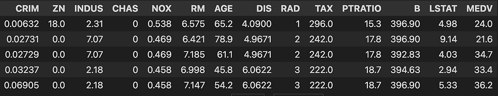
Linearity
Linearity is one of the key assumptions of linear regression, which states that the relationship between the independent variable(s) and the dependent variable should be linear. This means that the effect of changing the independent variable(s) on the dependent variable is constant across all levels of the independent variable(s).
However, in real-world datasets, the relationship between the independent and dependent variables may not always be linear. In such cases, the linear regression model may not provide accurate predictions. This is known as a violation of the linearity assumption.
There are several ways to address the violation of the linearity assumption in linear regression:
Non-linear transformations: One way to address the violation of the linearity assumption is to use non-linear transformations of the independent variable(s) to make the relationship more linear. For example, if the relationship between the independent and dependent variables is quadratic, we can add a squared term of the independent variable to the model.
Add interaction terms: Another way to address non-linearity is to add interaction terms between the independent variables. Interaction terms can capture the non-linear relationship between the independent variables and the dependent variable. An interaction term refers to a product term between two or more predictors (also known as independent variables) in the model. It represents the combined effect of the predictors on the dependent variable, and it allows the slope of one predictor to vary depending on the value of another predictor.
Generalized linear models: If the relationship between the independent and dependent variables is non-linear, we can use generalized linear models (GLMs) instead of linear regression. GLMs can model non-linear relationships by using different link functions and error distributions.
Let's take an example of aBoston Housing dataset from Kaggle, which contains information about various features of houses in Boston and their corresponding prices. One of the features in this dataset is the "RM" feature. We can plot the relationship between the "RM" feature and the "MDEV" variable using a scatter plot.
sns.regplot(x = dataframe['RM'] , y = dataframe['MEDV'])
plt.title("Relationship between RM and Price")
plt.xlabel("Number of rooms")
plt.ylabel("Price")
plt.show()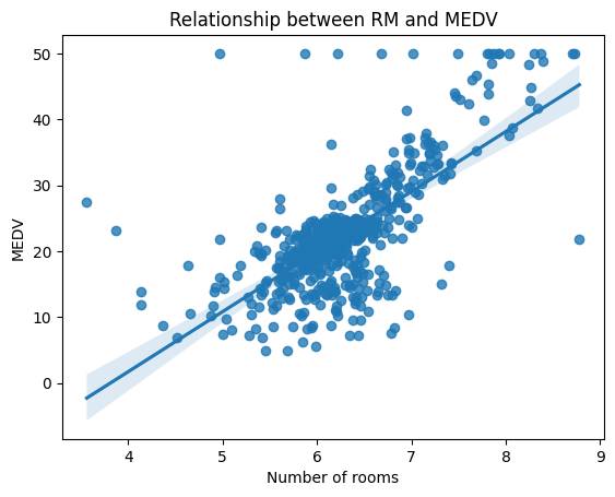
From the scatter plot, we can see that there is a positive relationship between the "RM" feature and the "MEDV" variable. However, the relationship does not appear to be strictly linear. This suggests that a simple linear regression model may not be the best fit for this data.
To address this issue, we can try transforming the variables to achieve a more linear relationship. One common transformation is taking the logarithm of the variables. We can apply this transformation to the "RM" variable and plot the transformed relationship using a scatter plot.
sns.regplot(x = np.log(dataframe['RM']) , y = dataframe['MEDV'])
plt.title("Relationship between log(RM) and MEDV")
plt.xlabel("Number of rooms")
plt.ylabel("MEDV")
plt.show()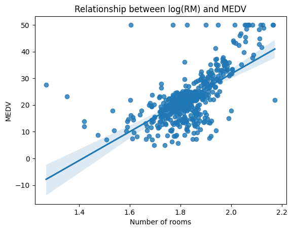
From the transformed scatter plot, we can see that the relationship between the "log(RM)" feature and the "MEDV" variable appears to be more linear (Once we deal with the outliers which is another interesting topic to cover). This suggests that a linear regression model using the transformed variables may be a better fit for this data.
Homoscedasticity
Homoscedasticity is an assumption of linear regression which states that the variance of the errors (i.e., the difference between the predicted values and the actual values) is constant across all levels of the predictor variable. In simpler terms, it means that the spread of the residuals should be roughly the same for all values of the predictor variable. If this assumption is violated, it can lead to biased or inefficient estimates of the regression coefficients and standard errors.
To check for homoscedasticity, one common method is to create a scatter plot of the residuals against the predicted values. Ideally, the scatter plot should show a random pattern with no discernible trend. However, if the spread of the residuals increases or decreases as the predicted values increase, this indicates that the assumption of homoscedasticity may be violated.
# loading the regression model
LR_model = LinearRegression()

# fitting trainin and testing dataset
LR_model.fit(X_train , y_train)

# predicting the target values
y_pred_train = LR_model.predict(X_train)
y_pred_test = LR_model.predict(X_test)

# Calculating Mean Squared error to analyse our model
mse_train = mean_squared_error(y_train, y_pred_train)
mse_test = mean_squared_error(y_test, y_pred_test)

# printing MSE
print("Training set MSE: ", mse_train) # 21.6414
print("Testing set MSE: ", mse_test) # 24.29111

# calculating residuals
residuals_train = y_train - y_pred_train
residuals_test = y_test - y_pred_test

#plotting for checking Homoscedasticity
plt.scatter(y_pred_train, residuals_train, label='Training Set')
plt.scatter(y_pred_test, residuals_test, label='Testing Set')
plt.axhline(y=0, color='r', linestyle='-')
plt.xlabel('Predicted Values')
plt.ylabel('Residuals')
plt.legend()
plt.show()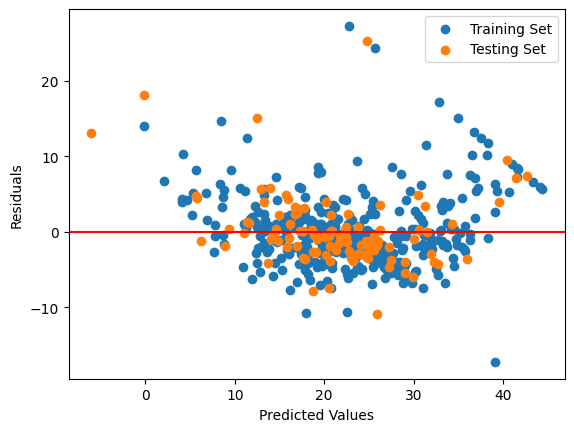
Since MSE values are high, indicating poor model performance. We generated scatter plot of the residuals against the predicted values to check for homoscedasticity. The resulting plot should show a scatter of points with a horizontal red line at y=0. Ideally, the points should be randomly scattered around the red line with no discernible trend but clearly the plot shows that the current regression model is not correct. So we need to correct something so that homoscedasticity condition holds. One way to solve this problem is to transform the dependent variable (i.e., the target variable) using a power transformation such as the natural logarithm or the square root (as done in linearity and check for same).
Multicollinearity
Multicollinearity is a common issue in linear regression where two or more predictor variables in a model are highly correlated, making it difficult to determine the individual effect of each variable on the target variable. This can lead to unreliable and unstable coefficient estimates, which can affect the overall performance of the model.
In order to detect multicollinearity, one can compute the correlation matrix of the predictor variables and look for high correlation coefficients. A commonly used threshold for high correlation is 0.7, although this may vary depending on the context and domain knowledge.
One way to solve the multicollinearity problem is to remove one or more of the correlated variables from the model. This can be done by using domain knowledge, or by using a feature selection method such as stepwise regression or Lasso regularization. Another approach is to use a dimensionality reduction technique such as Principal Component Analysis (PCA).
let's compute the correlation matrix of the Boston Dataset features
# calculating correlation matrix
corr_matrix = dataframe.corr()

# setting dimension of heatmap
plt.figure(figsize=(10,10))

# plotting the  matrix
sns.heatmap(corr_matrix , annot=True)
We can see that some pairs of features have high correlation coefficients, such as 'RAD' and 'TAX' (0.91), 'DIS' and 'AGE' (-0.75), and 'NOX' and 'INDUS' (0.76). This suggests that there might be multicollinearity in the dataset
To solve the multicollinearity problem, we can use PCA to reduce the dimensionality of the feature space. PCA works by finding the principal components that capture the most variance in the data, and projecting the data onto these components. This can help to remove the correlation between the original features and create new uncorrelated features that better explain the target variable.
# loading PCA
pca = PCA()

# first normalize every feature in dataset
X_norm = (X - X.mean()) / X.std()
X_pca = pca.fit_transform(X_norm)

# ploting the graph
plt.plot(pca.explained_variance_ratio_)
plt.xlabel('Number of Components')
plt.ylabel('Explained Variance Ratio')
plt.show()
We can see that the first few components capture most of the variance in the data, so we can use them as new features in our model by discarding some of low variance features.
Normality
Normality is one of the key assumptions in linear regression, which means that the residuals (the differences between the predicted values and the actual values) should be normally distributed. The assumption of normality is important because if the residuals are not normally distributed, it can lead to biased estimates of the regression coefficients and incorrect hypothesis testing results.
To check the normality assumption in linear regression, we can use a probability plot (also called a Q-Q plot) of the residuals, which is a scatter plot of the ordered residuals against the expected values from a normal distribution. If the residuals are normally distributed, the points on the probability plot should fall approximately along a straight line. Another way to check for normality is to use a histogram of the residuals, which should have a roughly bell-shaped distribution.
# fiting the dataset
LR_model.fit(X,y)

# predicting the dataset
y_pred = LR_model.predict(X)

# calculating residuals
residuals = y - y_pred

# Plot a probability plot of the residuals
probplot(residuals, plot=plt)
plt.show()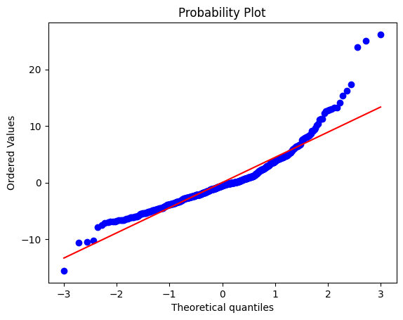
The resulting plot shows that the residuals deviate from a straight line, indicating that they are not normally distributed.
To address this issue, we can try transforming the response variable by taking the natural logarithm.
# applying log on target varible
y_log = np.log(y)

# fiting the dataset
LR_model.fit(X, y_log)

# predicting the dataset
y_log_pred = LR_model.predict(X)

# calculating residuals
residuals = y_log - y_log_pred

# Plot a probability plot of the residuals
probplot(residuals, plot=plt)
plt.show()
The resulting plot shows that the residuals are now approximately normally distributed.
There are many techniques to check whether the features holds the assumption or not. Ideally, this analysis is done to whole dataset and each feature is transformed so that most of the condition holds. You can try doing the same or you can do on this house price prediction dataset which can give you more complexity and knowledge about feature types.
A.N. : If you see any things that is incorrect, or you can add more to this post, or you wan to ask questions you can do that in comment or do you can connect with me here.


Comments